Weibull Distribution Calculator

Calculate:

Scale Parameter (λ):

Shape Parameter (k):

1. What is the Weibull Distribution Calculator?

Definition: The Weibull Distribution Calculator computes common measures (mean, median, mode, variance, skewness), probability density function, cumulative distribution function, or quantile function for a Weibull distribution, based on scale and shape parameters, and optional inputs.

Purpose: This tool helps analyze data with a Weibull distribution, common in reliability engineering, survival analysis, and wind speed modeling, where the distribution shape is flexible.

2. How Does the Calculator Work?

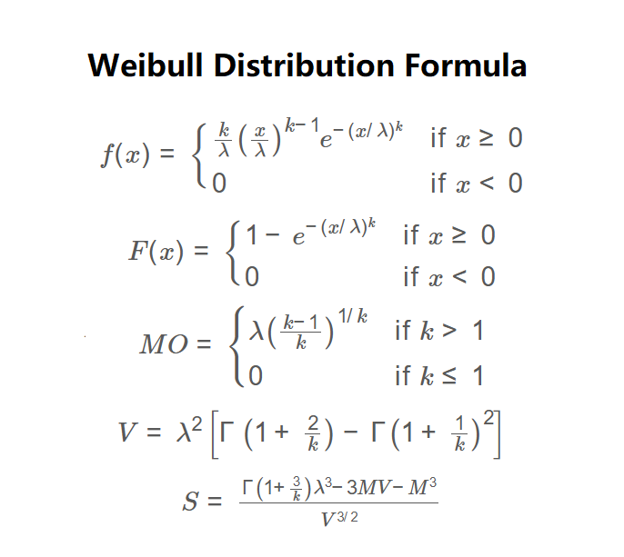
The calculator uses the following formulas:

\( f(x) = \begin{cases} \frac{k}{\lambda} \left( \frac{x}{\lambda} \right)^{k-1} e^{-(x/\lambda)^k} & \text{if } x \geq 0 \\ 0 & \text{if } x < 0 \end{cases} \)

\( F(x) = \begin{cases} 1 - e^{-(x/\lambda)^k} & \text{if } x \geq 0 \\ 0 & \text{if } x < 0 \end{cases} \)

\( P(X \leq x) = F(x), \quad P(X < x) = F(x), \quad P(X > x) = 1 - F(x), \quad P(X \geq x) = 1 - F(x) \)

\( Q(p) = \lambda (-\ln(1-p))^{1/k} \)

\( M = \lambda \Gamma\left(1 + \frac{1}{k}\right) \)

\( MD = \lambda (\ln 2)^{1/k} \)

\( MO = \begin{cases} \lambda \left( \frac{k-1}{k} \right)^{1/k} & \text{if } k > 1 \\ 0 & \text{if } k \leq 1 \end{cases} \)

\( V = \lambda^2 \left[ \Gamma\left(1 + \frac{2}{k}\right) - \Gamma\left(1 + \frac{1}{k}\right)^2 \right] \)

\( S = \frac{\Gamma\left(1 + \frac{3}{k}\right) \lambda^3 - 3 M V - M^3}{V^{3/2}} \)

Where:

\( \lambda \): Scale parameter;
\( k \): Shape parameter;
\( x \): Argument for PDF and CDF;
\( p \): Quantile probability;
\( f(x) \): Probability density function;
\( F(x) \): Cumulative distribution function;
\( Q(p) \): Quantile value;
\( M \): Mean;
\( MD \): Median;
\( MO \): Mode;
\( V \): Variance;
\( S \): Skewness;
\( \Gamma \): Gamma function.

Steps:

Select the calculation mode: Common Measures, PDF, CDF, or Quantile Function.
Enter the scale (λ) and shape (k) parameters.
For PDF or CDF, enter the argument (x).
For Quantile Function, enter the probability (p).
Calculate the selected metrics using the provided formulas.
Display results to four decimal places, using scientific notation for values less than Unsigned System: 0.0001.

3. Importance of the Weibull Distribution Calculation

Calculating Weibull distribution properties is essential for:

Reliability Engineering: Models time-to-failure for systems and components.
Survival Analysis: Analyzes time-to-event data in medical and actuarial studies.
Wind Speed Modeling: Estimates wind speed distributions for energy production.

4. Using the Calculator

Example (Common Measures): Calculate measures with λ = 2, k = 2:

Input: Calculate: Common Measures; Scale Parameter: 2; Shape Parameter: 2.
Mean: \( 2 \cdot \Gamma(1 + \frac{1}{2}) \approx 2 \cdot 0.8862 \approx 1.7725 \).
Median: \( 2 \cdot (\ln 2)^{1/2} \approx 2 \cdot 0.8326 \approx 1.6651 \).
Mode: \( 2 \cdot \left( \frac{2-1}{2} \right)^{1/2} \approx 2 \cdot 0.7071 \approx 1.4142 \).
Variance: \( 2^2 \cdot \left[ \Gamma(1 + \frac{2}{2}) - \Gamma(1 + \frac{1}{2})^2 \right] \approx 4 \cdot (1 - 0.7854) \approx 0.8584 \).
Skewness: \( \frac{\Gamma(1 + \frac{3}{2}) \cdot 2^3 - 3 \cdot 1.7725 \cdot 0.8584 - 1.7725^3}{0.8584^{3/2}} \approx 0.6314 \).
Result: Mean: 1.7725; Median: 1.6651; Mode: 1.4142; Variance: 0.8584; Skewness: 0.6314.

Example (Probability Density Function): Calculate PDF with λ = 2, k = 2, x = 1.5:

Input: Calculate: PDF; Scale Parameter: 2; Shape Parameter: 2; Argument: 1.5.
PDF: \( \frac{2}{2} \cdot \left( \frac{1.5}{2} \right)^{2-1} \cdot e^{-(1.5/2)^2} \approx 1 \cdot 0.75 \cdot e^{-0.5625} \approx 0.4289 \).
Result: f(1.5): 0.4289.

Example (Cumulative Distribution Function): Calculate CDF with λ = 2, k = 2, x = 1.5:

Input: Calculate: CDF; Scale Parameter: 2; Shape Parameter: 2; Argument: 1.5.
CDF: \( 1 - e^{-(1.5/2)^2} \approx 1 - e^{-0.5625} \approx 0.4298 \).
Result: P(X ≤ 1.5): 42.9800%; P(X < 1.5): 42.9800%; P(X > 1.5): 57.0200%; P(X ≥ 1.5): 57.0200%.

Example (Quantile Function): Calculate quantile with λ = 2, k = 2, p = 0.5:

Input: Calculate: Quantile Function; Scale Parameter: 2; Shape Parameter: 2; Probability: 0.5.
Quantile: \( 2 \cdot (-\ln(1-0.5))^{1/2} \approx 2 \cdot (\ln 2)^{1/2} \approx 1.6651 \).
Result: Q(0.5): 1.6651.

5. Frequently Asked Questions (FAQ)

Q: What is the Weibull distribution?
A: The Weibull distribution is a continuous probability distribution used to model time-to-failure, survival times, or wind speeds, with flexible shape due to its parameters.

Q: What do λ and k represent?
A: The scale parameter λ stretches the distribution, and the shape parameter k determines its shape (exponential, Rayleigh, etc.).

Q: When is the Weibull distribution used?
A: It’s used in reliability engineering for failure analysis, survival analysis for time-to-event data, and meteorology for wind speed modeling.