Lognormal Distribution Calculator

Calculate:

Mean of ln(X) (μ):

Standard Deviation of ln(X) (σ):

Mean (M):

Median (MD):

Mode (MO):

Variance (V):

Skewness (S):

1. What is the Lognormal Distribution Calculator?

Definition: The Lognormal Distribution Calculator computes either common measures (mean, median, mode, variance, skewness), the quantile function, the probability density function, or the cumulative distribution function of a lognormal distribution, based on the mean and standard deviation of the natural logarithm of the random variable, and an optional probability or argument.

Purpose: This tool helps analyze data with a lognormal distribution, common in finance, biology, and engineering, where the logarithm of the variable is normally distributed.

2. How Does the Calculator Work?

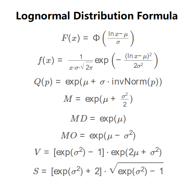
The calculator uses the following formulas:

\( F(x) = \Phi\left(\frac{\ln x - \mu}{\sigma}\right) \)

\( f(x) = \frac{1}{x \cdot \sigma \cdot \sqrt{2\pi}} \exp\left(-\frac{(\ln x - \mu)^2}{2\sigma^2}\right) \)

\( Q(p) = \exp(\mu + \sigma \cdot \text{invNorm}(p)) \)

\( M = \exp(\mu + \frac{\sigma^2}{2}) \)

\( MD = \exp(\mu) \)

\( MO = \exp(\mu - \sigma^2) \)

\( V = [\exp(\sigma^2) - 1] \cdot \exp(2\mu + \sigma^2) \)

\( S = [\exp(\sigma^2) + 2] \cdot \sqrt{\exp(\sigma^2) - 1} \)

Where:

\( x \): Argument for PDF and CDF;
\( p \): Quantile probability (0 to 1);
\( \mu \): Mean of ln(X);
\( \sigma \): Standard deviation of ln(X);
\( F(x) \): Cumulative distribution function;
\( f(x) \): Probability density function;
\( Q(p) \): Quantile value;
\( M \): Mean of X;
\( MD \): Median of X;
\( MO \): Mode of X;
\( V \): Variance of X;
\( S \): Skewness of X;
\( \Phi \): Standard normal CDF.

Steps:

Select the calculation mode: Common Measures, Quantile Function, Probability Density Function, or Cumulative Distribution Function.
Enter the mean (μ) and standard deviation (σ) of ln(X).
For Quantile Function mode, enter the quantile probability (p).
For Probability Density or Cumulative Distribution Function modes, enter the argument (x).
Calculate the selected metrics using the provided formulas.
Display results, using scientific notation for values with absolute value less than 0.0001, otherwise to four decimal places.

3. Importance of the Lognormal Distribution Calculation

Calculating lognormal distribution properties is essential for:

Financial Modeling: Models stock prices, asset returns, and other positively skewed financial data.
Scientific Analysis: Analyzes data in biology and engineering where variables are products of independent factors.
Risk Assessment: Assesses variability, asymmetry, quantiles, and probabilities in datasets with lognormal distributions.

4. Using the Calculator

Example (Common Measures): Calculate common measures with μ = 0, σ = 0.001:

Input: Calculate: Common Measures; Mean of ln(X): 0; Standard Deviation of ln(X): 0.001.
Mean: \( \exp(0 + \frac{0.001^2}{2}) = \exp(0.0000005) \approx 1.0000 \).
Median: \( \exp(0) = 1 \).
Mode: \( \exp(0 - 0.001^2) = \exp(-0.000001) \approx 9.999990e-1 \).
Variance: \( [\exp(0.001^2) - 1] \cdot \exp(2 \cdot 0 + 0.001^2) \approx 1.0000 \times 10^{-6} \approx 1.0000e-6 \).
Skewness: \( [\exp(0.001^2) + 2] \cdot \sqrt{\exp(0.001^2) - 1} \approx 3.0000 \times \sqrt{0.000001} \approx 3.0000e-3 \).
Result: Mean: 1.0000; Median: 1.0000; Mode: 9.999990e-1; Variance: 1.0000e-6; Skewness: 3.0000e-3.

Example (Quantile Function): Calculate the quantile with μ = 0, σ = 0.001, p = 0.95:

Input: Calculate: Quantile Function; Mean of ln(X): 0; Standard Deviation of ln(X): 0.001; Quantile Probability: 0.95.
Quantile: \( \exp(0 + 0.001 \cdot \text{invNorm}(0.95)) \approx \exp(0 + 0.001 \cdot 1.6449) \approx 1.0016 \).
Result: Quantile Q(0.95): 1.0016.

Example (Probability Density Function): Calculate the PDF with μ = 0, σ = 0.001, x = 1:

Input: Calculate: Probability Density Function; Mean of ln(X): 0; Standard Deviation of ln(X): 0.001; Argument: 1.
PDF: \( \frac{1}{1 \cdot 0.001 \cdot \sqrt{2\pi}} \exp\left(-\frac{(\ln 1 - 0)^2}{2 \cdot 0.001^2}\right) \approx 398.9423 \).
Result: Probability Density f(1): 398.9423.

Example (Cumulative Distribution Function): Calculate the CDF with μ = 0, σ = 0.001, x = 1:

Input: Calculate: Cumulative Distribution Function; Mean of ln(X): 0; Standard Deviation of ln(X): 0.001; Argument: 1.
CDF: \( \Phi\left(\frac{\ln 1 - 0}{0.001}\right) = \Phi(0) \approx 0.5000 \).
Result: Cumulative Probability F(1): 0.5000.

5. Frequently Asked Questions (FAQ)

Q: What is a lognormal distribution?
A: A lognormal distribution describes a random variable whose logarithm is normally distributed, common for positive, skewed data.

Q: What is the cumulative distribution function?
A: The CDF gives the probability that a random variable is less than or equal to a specific value, useful for understanding cumulative probabilities.

Q: Why are μ and σ based on ln(X)?
A: In a lognormal distribution, μ and σ represent the mean and standard deviation of the logarithm of the variable, not the variable itself.