Effective Duration Calculator

Face Value: dollars

Annual Coupon Rate: %

Coupon Frequency:

Years to Maturity: years

Yield to Maturity (YTM): %

Yield Differential: %

Coupon per Period:

dollars

Bond Price:

dollars

Upwards Bond Price (YTM - Yield Differential):

dollars

Downwards Bond Price (YTM + Yield Differential):

dollars

Effective Duration:

years

1. What is the Effective Duration Calculator?

Definition: This calculator computes the effective duration ($ ED $), a measure of a bond’s price sensitivity to changes in interest rates, accounting for changes in cash flows due to embedded options or yield shifts.

Purpose: Helps investors and portfolio managers assess interest rate risk, enabling better bond selection and risk management.

2. How Does the Calculator Work?

The calculator follows a four-step process to compute the effective duration:

Formulas:

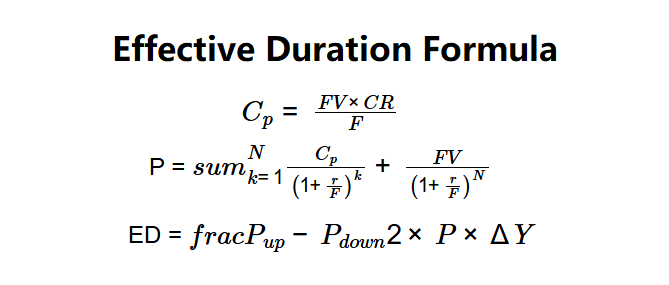
$ C_p = \frac{FV \times CR}{F} $

P = $sum_{k=1}^{N} \frac{C_p}{\left(1 + \frac{r}{F}\right)^k} + \frac{FV}{\left(1 + \frac{r}{F}\right)^N}$

Where $ r $ is $ YTM $, $ YTM - \Delta Y $, or $ YTM + \Delta Y $, and $ N = T \times F $.

ED = $frac{P_{up} - P_{down}}{2 \times P \times \Delta Y}$

Where:

$ ED $: Effective Duration (years)
$ C_p $: Coupon per Period (dollars)
$ P $: Bond Price at $ YTM $ (dollars)
$ P_{up} $: Bond Price at $ YTM - \Delta Y $ (dollars)
$ P_{down} $: Bond Price at $ YTM + \Delta Y $ (dollars)
$ FV $: Face Value (dollars)
$ CR $: Annual Coupon Rate (decimal)
$ F $: Coupon Frequency (per year)
$ T $: Years to Maturity
$ YTM $: Yield to Maturity (decimal)
$ \Delta Y $: Yield Differential (decimal)
$ N $: Total Periods ($ T \times F $)

Steps:

Step 1: Calculate coupon per period. Compute $ C_p = \frac{FV \times CR}{F} $.
Step 2: Calculate bond price. Compute $ P $ using $ YTM $.
Step 3: Calculate upwards and downwards bond prices. Compute $ P_{up} $ at $ YTM - \Delta Y $ and $ P_{down} $ at $ YTM + \Delta Y $.
Step 4: Calculate effective duration. Compute $ ED = \frac{P_{up} - P_{down}}{2 \times P \times \Delta Y} $.

3. Importance of Effective Duration Calculation

Calculating effective duration is crucial for:

Interest Rate Risk: Measures how a bond’s price changes with a 1% yield shift, critical for managing portfolio risk.
Bond Selection: Helps investors choose bonds with desired sensitivity to rate changes.
Portfolio Management: Enables balancing of interest rate exposure across bond holdings.

4. Using the Calculator

Example (Bond Alpha): $ FV = \$1,000 $, $ CR = 5\% $, $ F = 1 $, $ T = 10 $, $ YTM = 8\% $, $ \Delta Y = 1\% $:

Step 1: $ C_p = \frac{1,000 \times 0.05}{1} = \$50 $.
Step 2: $ P = \sum_{k=1}^{10} \frac{50}{(1 + 0.08)^k} + \frac{1,000}{(1 + 0.08)^{10}} = \$798.70 $.
Step 3:
- $ P_{up} = \sum_{k=1}^{10} \frac{50}{(1 + 0.07)^k} + \frac{1,000}{(1 + 0.07)^{10}} = \$859.53 $ (at $ YTM = 7\% $).
- $ P_{down} = \sum_{k=1}^{10} \frac{50}{(1 + 0.09)^k} + \frac{1,000}{(1 + 0.09)^{10}} = \$743.29 $ (at $ YTM = 9\% $).
Step 4: $ ED = \frac{859.53 - 743.29}{2 \times 798.70 \times 0.01} = \frac{116.24}{15.974} \approx 7.277 $.
Results: $ C_p = \$50 $, $ P = \$798.70 $, $ P_{up} = \$859.53 $, $ P_{down} = \$743.29 $, $ ED = 7.277 $ years.

An effective duration of 7.277 years indicates a 1% yield increase reduces the bond price by approximately 7.277%.

Example 2: $ FV = \$1,000 $, $ CR = 6\% $, $ F = 2 $, $ T = 5 $, $ YTM = 7\% $, $ \Delta Y = 0.5\% $:

Step 1: $ C_p = \frac{1,000 \times 0.06}{2} = \$30 $.
Step 2: $ P = \sum_{k=1}^{10} \frac{30}{(1 + \frac{0.07}{2})^k} + \frac{1,000}{(1 + \frac{0.07}{2})^{10}} \approx \$957.35 $.
Step 3:
- $ P_{up} = \sum_{k=1}^{10} \frac{30}{(1 + \frac{0.065}{2})^k} + \frac{1,000}{(1 + \frac{0.065}{2})^{10}} \approx \$981.22 $ (at $ YTM = 6.5\% $).
- $ P_{down} = \sum_{k=1}^{10} \frac{30}{(1 + \frac{0.075}{2})^k} + \frac{1,000}{(1 + \frac{0.075}{2})^{10}} \approx \$934.02 $ (at $ YTM = 7.5\% $).
Step 4: $ ED = \frac{981.22 - 934.02}{2 \times 957.35 \times 0.005} \approx \frac{47.20}{9.5735} \approx 4.931 $.
Results: $ C_p = \$30 $, $ P \approx \$957.35 $, $ P_{up} \approx \$981.22 $, $ P_{down} \approx \$934.02 $, $ ED \approx 4.931 $ years.

An effective duration of 4.931 years suggests moderate sensitivity to yield changes.

Example 3: $ FV = \$1,000 $, $ CR = 4\% $, $ F = 1 $, $ T = 15 $, $ YTM = 3\% $, $ \Delta Y = 1\% $:

Step 1: $ C_p = \frac{1,000 \times 0.04}{1} = \$40 $.
Step 2: $ P = \sum_{k=1}^{15} \frac{40}{(1 + 0.03)^k} + \frac{1,000}{(1 + 0.03)^{15}} \approx \$1,103.48 $.
Step 3:
- $ P_{up} = \sum_{k=1}^{15} \frac{40}{(1 + 0.02)^k} + \frac{1,000}{(1 + 0.02)^{15}} \approx \$1,172.07 $ (at $ YTM = 2\% $).
- $ P_{down} = \sum_{k=1}^{15} \frac{40}{(1 + 0.04)^k} + \frac{1,000}{(1 + 0.04)^{15}} \approx \$1,040.58 $ (at $ YTM = 4\% $).
Step 4: $ ED = \frac{1,172.07 - 1,040.58}{2 \times 1,103.48 \times 0.01} \approx \frac{131.49}{22.0696} \approx 5.957 $.
Results: $ C_p = \$40 $, $ P \approx \$1,103.48 $, $ P_{up} \approx \$1,172.07 $, $ P_{down} \approx \$1,040.58 $, $ ED \approx 5.957 $ years.

An effective duration of 5.957 years indicates a 1% yield change impacts the bond price by about 5.957%.

5. Frequently Asked Questions (FAQ)

Q: How does effective duration differ from Macaulay duration?
A: Effective duration accounts for changes in cash flows due to yield shifts (e.g., embedded options), while Macaulay duration assumes fixed cash flows.

Q: Why use a yield differential?
A: The yield differential ($ \Delta Y $) simulates small yield changes to estimate price sensitivity, ensuring accurate duration measurement.

Q: Can effective duration be negative?
A: Yes, for bonds with complex features (e.g., certain mortgage-backed securities), but rare for standard bonds like Bond Alpha.